Ever thought of getting started and wondered how would your first step is going to be? Well, Before you think, Start with at least Something.

Machine Learning : To develop Systems that would learn without extensive instructions. There are certain algorithms and rules that will help us extract information(patterns) from data.

Machine Learning is classified into 3 categories :

1. Supervised Machine Learning
2. Unsupervised Machine Learning
3. Semi-Supervised Machine Learning

Right now we'll be looking at a Supervised Machine Learning Algorithm. The Algorithm is called Linear Regression.

Linear Regression : The supervised Machine Learning model in which the model finds the best fit linear line between the independent and dependent variable.

Let's Understand with an Example, Let's say you have integer values and you stored them in an array. Now create another array with same number of values as the first array.

Array-1:

X = [45, 60, 20, 66, 32, 46, 18, 65, 15, 70]

Array-2:

Y = [55, 75, 31, 76, 44, 59, 33, 70, 26, 83]

Now, we will input an integer value to the Linear Regression Algorithm, and it will predict a value according to how the values get fitted in the algorithm.

Libraries For this task we'll be using basic libraries

1. Numpy
2. Matplotlib
3. Sklearn

Steps:

Step-1: Import the libraries:

import numpy as np
import matplotlib.pyplot as plt
from sklearn.linear_model import LinearRegression
from sklearn.model_selection import train_test_split

Step-2: Import the dataset:

X = np.array([45, 60, 20, 66, 32, 46, 18, 65, 15, 70]).reshape(-1,1)

Y = np.array([55, 75, 31, 76, 44, 59, 33, 70, 26, 83]).reshape(-1,1)

Step-3: Using the train_test_split() function from sklearn

x_train, x_test, y_train, y_train = train_test_split(X, Y, test_size=0.1)

Step-4: Fit the model:

model = LinearRegression()
model.fit(X, Y)

Step-5: calculating the Accuracy of our model:

model.score(X, Y)

Score : 0.9816145767514913

Step-6: Plotting the datapoints and visualizing it through a scatter plot

plt.scatter(X, Y)
plt.plot(np.linspace(0,70,100).reshape(-1,1), model.predict(np.linspace(0,70,100).reshape(-1,1)),'r')
plt.show()

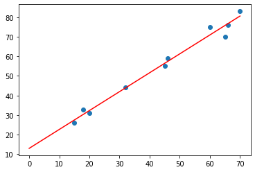
Scatter Plot: Representation of the X and Y DataPoints in a plane. The Red Line is the representation that the Linear Regression Model is fitted wrt the datapoints.

Step-7: Predicting new values:

x_arr = np.array([int(input("Enter a value : "))]).reshape(-1,1)
x_new = np.array([x_arr]).reshape(-1,1)
y_predict = model.predict(x_new)
print(y_predict)

Enter a value : 65

Predicted Value: 75.75415436

This is a Basic Linear Regression model to understand how the model is fitted, How the values are set, and how the Predictions are performed.